性别与智商的关系

回到脑容量 + 智商数据，在去除脑容量、身高和体重的影响后，测试男性和女性的言语智商 (VIQ) 是否存在差异。

注意，这里“性别”是一个类别值。由于它是非浮点型数据，statsmodels 可以自动推断这一点。

import pandas
from statsmodels.formula.api import ols

data = pandas.read_csv("../brain_size.csv", sep=";", na_values=".")

model = ols("VIQ ~ Gender + MRI_Count + Height", data).fit()
print(model.summary())

# Here, we don't need to define a contrast, as we are testing a single
# coefficient of our model, and not a combination of coefficients.
# However, defining a contrast, which would then be a 'unit contrast',
# will give us the same results
print(model.f_test([0, 1, 0, 0]))

                            OLS Regression Results
==============================================================================
Dep. Variable:                    VIQ   R-squared:                       0.246
Model:                            OLS   Adj. R-squared:                  0.181
Method:                 Least Squares   F-statistic:                     3.809
Date:                Mon, 07 Oct 2024   Prob (F-statistic):             0.0184
Time:                        04:57:10   Log-Likelihood:                -172.34
No. Observations:                  39   AIC:                             352.7
Df Residuals:                      35   BIC:                             359.3
Df Model:                           3
Covariance Type:            nonrobust
==================================================================================
                     coef    std err          t      P>|t|      [0.025      0.975]
----------------------------------------------------------------------------------
Intercept        166.6258     88.824      1.876      0.069     -13.696     346.948
Gender[T.Male]     8.8524     10.710      0.827      0.414     -12.890      30.595
MRI_Count          0.0002   6.46e-05      2.615      0.013    3.78e-05       0.000
Height            -3.0837      1.276     -2.417      0.021      -5.674      -0.494
==============================================================================
Omnibus:                        7.373   Durbin-Watson:                   2.109
Prob(Omnibus):                  0.025   Jarque-Bera (JB):                2.252
Skew:                           0.005   Prob(JB):                        0.324
Kurtosis:                       1.823   Cond. No.                     2.40e+07
==============================================================================

Notes:
[1] Standard Errors assume that the covariance matrix of the errors is correctly specified.
[2] The condition number is large, 2.4e+07. This might indicate that there are
strong multicollinearity or other numerical problems.
<F test: F=0.683196084584229, p=0.4140878441244694, df_denom=35, df_num=1>

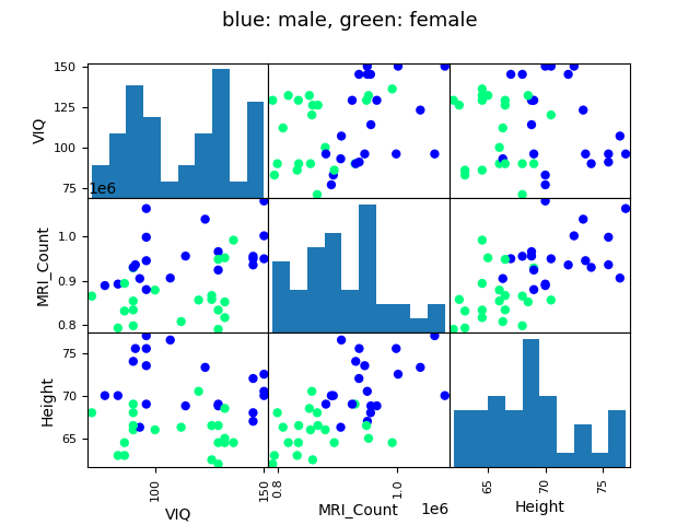
这里我们绘制散点矩阵以获得对结果的直观认识。这超出了练习中要求的内容。

# This plotting is useful to get an intuitions on the relationships between
# our different variables

from pandas import plotting
import matplotlib.pyplot as plt

# Fill in the missing values for Height for plotting
data["Height"] = data["Height"].ffill()

# The parameter 'c' is passed to plt.scatter and will control the color
# The same holds for parameters 'marker', 'alpha' and 'cmap', that
# control respectively the type of marker used, their transparency and
# the colormap
plotting.scatter_matrix(
    data[["VIQ", "MRI_Count", "Height"]],
    c=(data["Gender"] == "Female"),
    marker="o",
    alpha=1,
    cmap="winter",
)

fig = plt.gcf()
fig.suptitle("blue: male, green: female", size=13)

plt.show()