3.1.6.6. 工资中的教育/性别交互作用测试

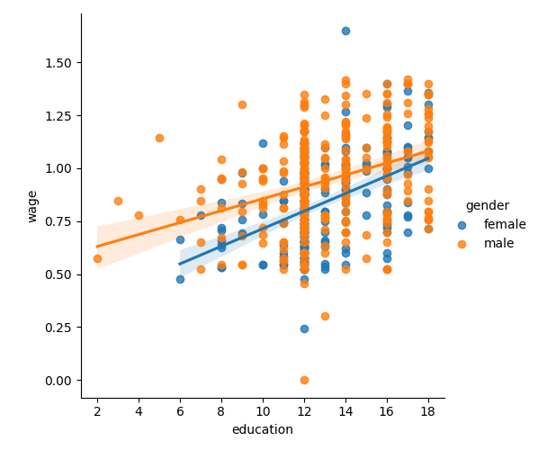
工资主要取决于教育水平。在这里，我们调查这种依赖关系与性别的关系：性别不仅会在工资中产生偏移，而且工资随着教育水平的提高而增加的速度似乎也比女性更高。

我们的数据是否支持最后这个假设？我们将使用 statsmodels 的公式（http://statsmodels.sourceforge.net/stable/example_formulas.html）来测试这一点。

加载和处理数据

import pandas

import urllib.request
import os

if not os.path.exists("wages.txt"):
    # Download the file if it is not present
    url = "http://lib.stat.cmu.edu/datasets/CPS_85_Wages"
    with urllib.request.urlopen(url) as r, open("wages.txt", "wb") as f:
        f.write(r.read())

# EDUCATION: Number of years of education
# SEX: 1=Female, 0=Male
# WAGE: Wage (dollars per hour)
data = pandas.read_csv(
    "wages.txt",
    skiprows=27,
    skipfooter=6,
    sep=None,
    header=None,
    names=["education", "gender", "wage"],
    usecols=[0, 2, 5],
)

# Convert genders to strings (this is particularly useful so that the
# statsmodels formulas detects that gender is a categorical variable)
import numpy as np

data["gender"] = np.choose(data.gender, ["male", "female"])

# Log-transform the wages, because they typically are increased with
# multiplicative factors
data["wage"] = np.log10(data["wage"])

/home/runner/work/scientific-python-lectures/scientific-python-lectures/packages/statistics/examples/plot_wage_education_gender.py:32: ParserWarning: Falling back to the 'python' engine because the 'c' engine does not support skipfooter; you can avoid this warning by specifying engine='python'.
  data = pandas.read_csv(

简单的绘图

import seaborn

# Plot 2 linear fits for male and female.
seaborn.lmplot(y="wage", x="education", hue="gender", data=data)

<seaborn.axisgrid.FacetGrid object at 0x7f78e72a34a0>

统计分析

import statsmodels.formula.api as sm

# Note that this model is not the plot displayed above: it is one
# joined model for male and female, not separate models for male and
# female. The reason is that a single model enables statistical testing
result = sm.ols(formula="wage ~ education + gender", data=data).fit()
print(result.summary())

                            OLS Regression Results
==============================================================================
Dep. Variable:                   wage   R-squared:                       0.193
Model:                            OLS   Adj. R-squared:                  0.190
Method:                 Least Squares   F-statistic:                     63.42
Date:                Mon, 07 Oct 2024   Prob (F-statistic):           2.01e-25
Time:                        04:56:52   Log-Likelihood:                 86.654
No. Observations:                 534   AIC:                            -167.3
Df Residuals:                     531   BIC:                            -154.5
Df Model:                           2
Covariance Type:            nonrobust
==================================================================================
                     coef    std err          t      P>|t|      [0.025      0.975]
----------------------------------------------------------------------------------
Intercept          0.4053      0.046      8.732      0.000       0.314       0.496
gender[T.male]     0.1008      0.018      5.625      0.000       0.066       0.136
education          0.0334      0.003      9.768      0.000       0.027       0.040
==============================================================================
Omnibus:                        4.675   Durbin-Watson:                   1.792
Prob(Omnibus):                  0.097   Jarque-Bera (JB):                4.876
Skew:                          -0.147   Prob(JB):                       0.0873
Kurtosis:                       3.365   Cond. No.                         69.7
==============================================================================

Notes:
[1] Standard Errors assume that the covariance matrix of the errors is correctly specified.

上面的图突出了工资不仅存在不同的偏移，而且斜率也不同。

我们需要使用交互作用来建模。

result = sm.ols(
    formula="wage ~ education + gender + education * gender", data=data
).fit()
print(result.summary())

                            OLS Regression Results
==============================================================================
Dep. Variable:                   wage   R-squared:                       0.198
Model:                            OLS   Adj. R-squared:                  0.194
Method:                 Least Squares   F-statistic:                     43.72
Date:                Mon, 07 Oct 2024   Prob (F-statistic):           2.94e-25
Time:                        04:56:52   Log-Likelihood:                 88.503
No. Observations:                 534   AIC:                            -169.0
Df Residuals:                     530   BIC:                            -151.9
Df Model:                           3
Covariance Type:            nonrobust
============================================================================================
                               coef    std err          t      P>|t|      [0.025      0.975]
--------------------------------------------------------------------------------------------
Intercept                    0.2998      0.072      4.173      0.000       0.159       0.441
gender[T.male]               0.2750      0.093      2.972      0.003       0.093       0.457
education                    0.0415      0.005      7.647      0.000       0.031       0.052
education:gender[T.male]    -0.0134      0.007     -1.919      0.056      -0.027       0.000
==============================================================================
Omnibus:                        4.838   Durbin-Watson:                   1.825
Prob(Omnibus):                  0.089   Jarque-Bera (JB):                5.000
Skew:                          -0.156   Prob(JB):                       0.0821
Kurtosis:                       3.356   Cond. No.                         194.
==============================================================================

Notes:
[1] Standard Errors assume that the covariance matrix of the errors is correctly specified.

观察性别和教育交互作用的 p 值，数据不支持教育对男性比女性更有利的假设（p 值 > 0.05）。

import matplotlib.pyplot as plt

plt.show()