3.4.8.15. 线性模型和非线性模型示例

这是一个来自教程的示例图，其中包含对支持向量机 GUI 的解释。

import numpy as np
import matplotlib.pyplot as plt

from sklearn import svm


rng = np.random.default_rng(27446968)

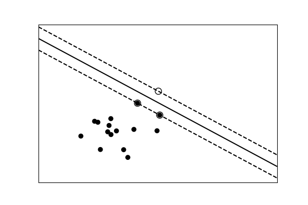
线性可分离的数据

def linear_model(rseed=42, n_samples=30):
    "Generate data according to a linear model"
    np.random.seed(rseed)

    data = np.random.normal(0, 10, (n_samples, 2))
    data[: n_samples // 2] -= 15
    data[n_samples // 2 :] += 15

    labels = np.ones(n_samples)
    labels[: n_samples // 2] = -1

    return data, labels


X, y = linear_model()
clf = svm.SVC(kernel="linear")
clf.fit(X, y)

plt.figure(figsize=(6, 4))
ax = plt.subplot(111, xticks=[], yticks=[])
ax.scatter(X[:, 0], X[:, 1], c=y, cmap="bone")

ax.scatter(
    clf.support_vectors_[:, 0],
    clf.support_vectors_[:, 1],
    s=80,
    edgecolors="k",
    facecolors="none",
)

delta = 1
y_min, y_max = -50, 50
x_min, x_max = -50, 50
x = np.arange(x_min, x_max + delta, delta)
y = np.arange(y_min, y_max + delta, delta)
X1, X2 = np.meshgrid(x, y)
Z = clf.decision_function(np.c_[X1.ravel(), X2.ravel()])
Z = Z.reshape(X1.shape)

ax.contour(
    X1, X2, Z, [-1.0, 0.0, 1.0], colors="k", linestyles=["dashed", "solid", "dashed"]
)

<matplotlib.contour.QuadContourSet object at 0x7f78e72a1d60>

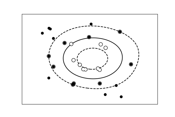
具有非线性分离的数据

def nonlinear_model(rseed=27446968, n_samples=30):
    rng = np.random.default_rng(rseed)

    radius = 40 * rng.random(n_samples)
    far_pts = radius > 20
    radius[far_pts] *= 1.2
    radius[~far_pts] *= 1.1

    theta = rng.random(n_samples) * np.pi * 2

    data = np.empty((n_samples, 2))
    data[:, 0] = radius * np.cos(theta)
    data[:, 1] = radius * np.sin(theta)

    labels = np.ones(n_samples)
    labels[far_pts] = -1

    return data, labels


X, y = nonlinear_model()
clf = svm.SVC(kernel="rbf", gamma=0.001, coef0=0, degree=3)
clf.fit(X, y)

plt.figure(figsize=(6, 4))
ax = plt.subplot(1, 1, 1, xticks=[], yticks=[])
ax.scatter(X[:, 0], X[:, 1], c=y, cmap="bone", zorder=2)

ax.scatter(
    clf.support_vectors_[:, 0],
    clf.support_vectors_[:, 1],
    s=80,
    edgecolors="k",
    facecolors="none",
)

delta = 1
y_min, y_max = -50, 50
x_min, x_max = -50, 50
x = np.arange(x_min, x_max + delta, delta)
y = np.arange(y_min, y_max + delta, delta)
X1, X2 = np.meshgrid(x, y)
Z = clf.decision_function(np.c_[X1.ravel(), X2.ravel()])
Z = Z.reshape(X1.shape)

ax.contour(
    X1,
    X2,
    Z,
    [-1.0, 0.0, 1.0],
    colors="k",
    linestyles=["dashed", "solid", "dashed"],
    zorder=1,
)

plt.show()