1.5.12.9. 声谱图，功率谱密度

演示在频率线性调频信号上的声谱图和功率谱密度。

import numpy as np
import matplotlib.pyplot as plt

生成线性调频信号

# Seed the random number generator
np.random.seed(0)

time_step = 0.01
time_vec = np.arange(0, 70, time_step)

# A signal with a small frequency chirp
sig = np.sin(0.5 * np.pi * time_vec * (1 + 0.1 * time_vec))

plt.figure(figsize=(8, 5))
plt.plot(time_vec, sig)

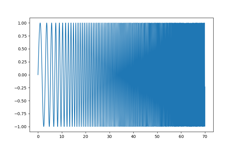
[<matplotlib.lines.Line2D object at 0x7f791eb0e480>]

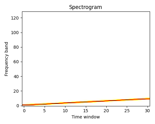
计算并绘制声谱图

信号在连续时间窗口上的频谱

import scipy as sp

freqs, times, spectrogram = sp.signal.spectrogram(sig)

plt.figure(figsize=(5, 4))
plt.imshow(spectrogram, aspect="auto", cmap="hot_r", origin="lower")
plt.title("Spectrogram")
plt.ylabel("Frequency band")
plt.xlabel("Time window")
plt.tight_layout()

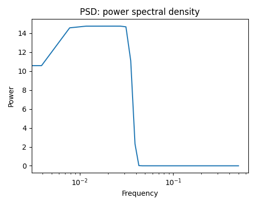
计算并绘制功率谱密度 (PSD)

信号在每个频段上的功率

freqs, psd = sp.signal.welch(sig)

plt.figure(figsize=(5, 4))
plt.semilogx(freqs, psd)
plt.title("PSD: power spectral density")
plt.xlabel("Frequency")
plt.ylabel("Power")
plt.tight_layout()

plt.show()