2.7.4.9. 交替优化

这里的挑战在于问题的 Hessian 矩阵是一个病态矩阵。这很容易看出来，因为第一项的 Hessian 矩阵仅仅是 2 * K.T @ K。因此，可以通过观察 K 的条件数来判断问题的条件数。

import time

import numpy as np
import scipy as sp
import matplotlib.pyplot as plt

rng = np.random.default_rng(27446968)

K = rng.normal(size=(100, 100))


def f(x):
    return np.sum((K @ (x - 1)) ** 2) + np.sum(x**2) ** 2


def f_prime(x):
    return 2 * K.T @ K @ (x - 1) + 4 * np.sum(x**2) * x


def hessian(x):
    H = 2 * K.T @ K + 4 * 2 * x * x[:, np.newaxis]
    return H + 4 * np.eye(H.shape[0]) * np.sum(x**2)

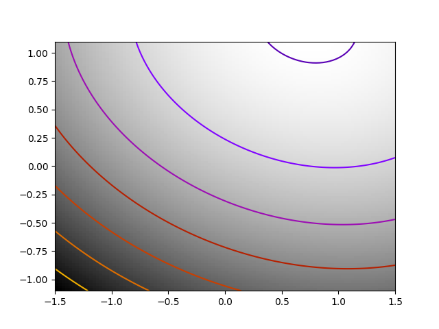
一些漂亮的绘图

plt.figure(1)
plt.clf()
Z = X, Y = np.mgrid[-1.5:1.5:100j, -1.1:1.1:100j]  # type: ignore[misc]
# Complete in the additional dimensions with zeros
Z = np.reshape(Z, (2, -1)).copy()
Z.resize((100, Z.shape[-1]))
Z = np.apply_along_axis(f, 0, Z)
Z = np.reshape(Z, X.shape)
plt.imshow(Z.T, cmap="gray_r", extent=(-1.5, 1.5, -1.1, 1.1), origin="lower")
plt.contour(X, Y, Z, cmap="gnuplot")

# A reference but slow solution:
t0 = time.time()
x_ref = sp.optimize.minimize(f, K[0], method="Powell").x
print(f"     Powell: time {time.time() - t0:.2f}s")
f_ref = f(x_ref)

# Compare different approaches
t0 = time.time()
x_bfgs = sp.optimize.minimize(f, K[0], method="BFGS").x
print(
    f"       BFGS: time {time.time() - t0:.2f}s, x error {np.sqrt(np.sum((x_bfgs - x_ref) ** 2)):.2f}, f error {f(x_bfgs) - f_ref:.2f}"
)

t0 = time.time()
x_l_bfgs = sp.optimize.minimize(f, K[0], method="L-BFGS-B").x
print(
    f"     L-BFGS: time {time.time() - t0:.2f}s, x error {np.sqrt(np.sum((x_l_bfgs - x_ref) ** 2)):.2f}, f error {f(x_l_bfgs) - f_ref:.2f}"
)


t0 = time.time()
x_bfgs = sp.optimize.minimize(f, K[0], jac=f_prime, method="BFGS").x
print(
    f"  BFGS w f': time {time.time() - t0:.2f}s, x error {np.sqrt(np.sum((x_bfgs - x_ref) ** 2)):.2f}, f error {f(x_bfgs) - f_ref:.2f}"
)

t0 = time.time()
x_l_bfgs = sp.optimize.minimize(f, K[0], jac=f_prime, method="L-BFGS-B").x
print(
    f"L-BFGS w f': time {time.time() - t0:.2f}s, x error {np.sqrt(np.sum((x_l_bfgs - x_ref) ** 2)):.2f}, f error {f(x_l_bfgs) - f_ref:.2f}"
)

t0 = time.time()
x_newton = sp.optimize.minimize(
    f, K[0], jac=f_prime, hess=hessian, method="Newton-CG"
).x
print(
    f"     Newton: time {time.time() - t0:.2f}s, x error {np.sqrt(np.sum((x_newton - x_ref) ** 2)):.2f}, f error {f(x_newton) - f_ref:.2f}"
)

plt.show()

     Powell: time 0.13s
       BFGS: time 0.80s, x error 0.02, f error -0.03
     L-BFGS: time 0.06s, x error 0.02, f error -0.03
  BFGS w f': time 0.06s, x error 0.02, f error -0.03
L-BFGS w f': time 0.00s, x error 0.02, f error -0.03
     Newton: time 0.00s, x error 0.02, f error -0.03